Every Layer a Store
The open frontier, part 1: how the 2026 open models are built
This is the first of two essays on the open-weight language models of 2026. It covers how they are built. The second covers how they are trained.
Give a language model a prompt of a million tokens. The picture most people carry of a Transformer says what happens next: every layer keeps an entry for every token, and every new token reads all of them. Most of this year’s large open models accept a prompt that long. Here are three, and none of them works that way.
MiMo-V2.6-Pro, from Xiaomi, has 70 layers. In 60 of them, each position looks back only 128 tokens. Ten layers see the whole prompt.
Kimi K3, from Moonshot, has 93 layers. Sixty-nine of them keep no per-token record at all. Each keeps a fixed-size matrix per head, and every token of the prompt updates that matrix and moves on. The other 24 layers keep their entries, compressed.
DeepSeek-V4.1-Flash has 40 layers, split into a 20-layer encoder and a 20-layer decoder. Most of the prompt passes only through the encoder. The decoder’s record of the prompt is projected from the encoder’s final states, and only the prompt’s last 128 tokens and the tokens the model generates pass through all 40 layers.
So where did the prompt go? Into stores of different kinds, each with its own way of writing, keeping and reading. Every layer of a Transformer is a memory. The 2026 open models extend the Transformer by choosing which memories to have, how each keeps its entries from interfering, and what reading them costs. Seven checkpoints carry the argument: the three above, Qwen3.8 from Alibaba, GLM-5.3 from Z.ai, DeepSeek-V4-Pro, and MiniMax-M3.
1. From the 2017 Transformer to today’s layer
The model of Attention Is All You Need was a translation system with an encoder and a decoder. It normalized after each residual addition and added position information to the input embeddings. The decoder-only, pre-normalized model that people now call “the Transformer” is a later descendant.
Attention is a lookup. Each position computes a query, a key and a value. A query is compared with the keys of the positions it may see. A softmax turns the comparisons into weights, and the output is the weighted average of the values:
\operatorname{Attention}(Q,K,V)=\operatorname{softmax}\!\left(\frac{QK^\top}{\sqrt{d_k}}+M\right)V .
The mask M hides the positions a query may not see, which in a language model are the future ones. Several heads run in parallel, each with its own projections. The word “head” is best read by analogy with the reading head of a tape. The Neural Turing Machine of 2014 had attention-based read and write heads. Attention Is All You Need does not explain its choice of word. It has nothing to do with the head of a phrase in syntax. In the recurrent layers of Section 3 the analogy becomes literal, since each head both writes to and reads from a memory of its own.
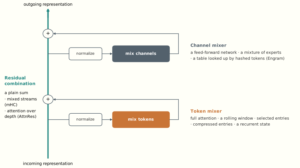
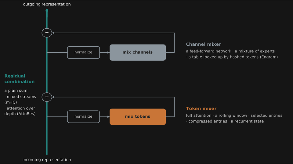
A Transformer is a stack of layers, repeated units with the same outline: when we say that Kimi K3 has 93 layers, we mean 93 of these units. Each layer combines two blocks, components such as an attention block or a feed-forward block, with wiring around them. The wiring normalizes each block’s input and adds the block’s output back to what came in, the residual addition. A modern layer thus has three slots:
incoming representation
  → normalize → mix tokens   → add to the residual
  → normalize → mix channels → add to the residual
  → outgoing representation
The token mixer moves information between positions; attention is the classic choice. The channel mixer transforms each position on its own; a feed-forward network is the classic choice. The residual combination carries each position’s representation from one layer to the next. Every model in this essay replaces at least one of the three.
Four smaller changes are common to most of them:
- RMSNorm rescales activations without subtracting their mean.
- Gated feed-forward networks such as SwiGLU multiply two projections of the input, one passed through a smooth nonlinearity.
- Rotary position embeddings rotate queries and keys so that their dot product depends on relative position. Not every model uses them: Kimi K3’s attention layers use none, and its recurrent layers carry the sense of order.
- Two devices shrink what attention keeps per token. Grouped-query attention lets several query heads share one key and value head. Multi-head latent attention (MLA) stores a compressed latent from which keys and values are reconstructed.
The largest change is conditional computation. A mixture of experts (MoE) replaces the single feed-forward network with many, and a router sends each token to a few. All seven models are MoE models. Kimi K3 stores 2.8 trillion parameters and uses 104 billion for each token.
Conditional computation makes it necessary to keep four quantities apart: the weights a model stores, the computation each token uses, the state a context occupies, and the time a piece of hardware takes. “Active parameters” measures only the second. It says nothing about memory, about the cost of a long context, or about speed.
2. Every layer is a store
Alex Wang recently gave a compact derivation of the Transformer’s layers as memories, building on Zhong and colleagues. It supplies the four questions this essay asks of every component: what writes the store, when, how much it holds before its entries interfere, and what reading it costs.
The outer-product store
Store pairs of vectors, a key k_i and a value v_i, by adding their outer products into one matrix:
W=\sum_i v_i k_i^\top .
To recall the value stored under key k_j, multiply:
Wk_j=v_j\,(k_j^\top k_j)+\sum_{i\neq j}v_i\,(k_i^\top k_j).
With unit-length keys the first term is the stored value. The sum is interference: every other value, weighted by how much its key overlaps the query. If the keys are random vectors in d dimensions, each overlap is about \pm d^{-1/2}, and the M-1 terms add up like a random walk. The interference grows as (M/d)^{1/2} relative to the signal, and it matches the signal at about M=d. A d\times d matrix written this way recalls about d random associations as clean vectors.
The linear associative memory. The outer-product store is half a century old. Teuvo Kohonen and James Anderson published it independently in 1972. Kohonen showed that recall is perfect when the keys are orthogonal and named the “crosstalk” that non-orthogonal keys produce. Anderson, writing about neurons, computed a signal-to-noise ratio that falls with the number of stored traces. Neither gave a capacity number. The first one came a year later. Kohonen and Ruohonen replaced the sum of outer products with the pseudo-inverse of the key matrix. That map recalls every stored value exactly when the keys are linearly independent, so for arbitrary values it stores at most as many pairs as the keys have dimensions. Beyond that it returns the least-squares approximation. An online route to the same map is older still. In 1960, Bernard Widrow and Ted Hoff trained an adaptive linear unit by measuring its error on one pattern at a time and moving each weight against the gradient of that error. Section 3 meets their rule again, inside Kimi K3 and Qwen3.8.
The least-squares store does better than the outer-product store, though not by much. It cancels the interference of correlated keys, recalls exactly up to d pairs, and in Wang’s estimate reaches the same interference-to-signal ratio as the outer-product store at about 2d pairs.
Nonlinearity suppresses interference
A feed-forward network computes
f(x)=\sum_i v_i\,\sigma(k_i^\top x),
which is the outer-product store with a nonlinearity \sigma applied to each overlap before it weights a value. The rows of the first weight matrix are keys and the columns of the second are values. A ReLU zeroes the negative overlaps, so about half the interfering terms vanish. That buys a factor of two. Squaring after the ReLU does far more. Small overlaps become very small, the stored key’s overlap of 1 stays 1, and the capacity grows to about 2d^2/3: some 2,700 pairs at d=64. A gated unit with a tied gate behaves the same way. Raising the overlap to the power p gives capacity of order d^p.
That feed-forward layers store associations this way is more than an analogy. A version of Attention Is All You Need already replaced the feed-forward layers with attention over learned key–value pairs, at about the same translation quality. Later versions dropped the passage. Sukhbaatar and colleagues folded such learned pairs into self-attention itself and removed the feed-forward layers without loss. Geva and colleagues took a trained 16-layer language model and looked at what the keys of its feed-forward layers respond to. For 65 to 80 percent of the inputs that most activate a key, annotators found a shared pattern: shallow ones, such as a common last word, in the lower layers, and semantic ones in the upper layers.
Hopfield and the 0.14 N limit. In 1982 John Hopfield stored patterns in a network of binary neurons with outer-product weights and let the network settle from a corrupted cue. From simulations with up to 100 neurons he reported that “about 0.15 N states can be simultaneously remembered before error in recall is severe”: at that load about half the memories were lost. Amit, Gutfreund and Sompolinsky derived the limit in 1985 with the tools of spin-glass physics: retrieval states exist up to 0.138N patterns, and at that load 1.5 percent of their bits are wrong. Demand exact recall and the count falls. McEliece and colleagues showed that most memories are recovered exactly up to about N/(2\log N), and all of them only up to N/(4\log N). Change the learning rule and the count rises. Elizabeth Gardner computed the capacity of the best possible couplings, whatever rule finds them, and got 2N. Error-correcting rules of the perceptron type reach it, and Hebb’s rule does not. Between these results the number of stored patterns moves by a logarithmic factor and more, depending on what counts as remembering and how the weights were set.
Dense associative memory. In 2016 Dmitry Krotov and John Hopfield generalized the energy of the Hopfield network so that each overlap enters through a power n. With small recall errors allowed, the capacity grows as N^{n-1}, and n=2 recovers the classical 0.14 N. Wang’s power p is their n-1. Demircigil and colleagues proved that an exponential energy gives a capacity exponential in N: 2^{N/2} patterns can be fixed points. Ramsauer and colleagues carried the exponential version over to continuous patterns and showed that its update rule is Transformer attention.
Softmax attention uses every power
The exponential is a sum of all the powers: e^{\beta s}=\sum_p(\beta s)^p/p!. Let a store weight each value by e^{\beta s}, where s is the overlap of its key with the query and \beta sets the sharpness. It suppresses interference more than any single power does. Normalize the weights by their sum, and the store is softmax attention:
f(q)=\sum_i v_i\,\frac{e^{\beta k_i^\top q}}{\sum_j e^{\beta k_j^\top q}} .
Wang’s estimate for random keys gives a capacity of about e^{2\beta(1-\beta/d)}. With the usual sharpness, \beta=d^{1/2}, that is about 1.2 million pairs at d=64.
Attention is a different kind of store from the feed-forward layer. Nothing is trained into it. Its keys and values are computed from the context while the model reads, and its M is the number of positions it sees. The feed-forward layer is written by training and holds what the model knows; the attention cache is written by reading and holds what the model has been told.
Sparse distributed memory. Pentti Kanerva’s model of 1988, described in his later summary, places about a million “hard locations” at random addresses in a space of 1,000-bit words. Writing a word at an address adds it to every location within a fixed Hamming distance of that address. Reading at an address sums the locations within that distance and takes a majority vote. Seen as a network, it has two layers: a fixed random first layer that decides which locations an address activates, and a second layer of counters. Its capacity grows with the number of locations, not with the word size. Kanerva’s practical guide was to store 1 to 5 percent as many words as there are locations. Bricken and Pehlevan showed that attention approximates its read operation when keys and queries are normalized to unit length and the sharpness is suitable. So the thresholded store of a feed-forward layer and the exponential store of attention have a classical model between them. Sparse distributed memory also bears on a current debate in interpretability, about whether a network’s neurons are clean. With random addresses, one location holds unrelated items by design. When Bricken and colleagues let a sparse distributed memory learn its addresses under the right constraints, its units specialized to classes of inputs instead.
What counts as remembering
All these numbers count clean recall: the recalled vector must be closer to the stored value than the interference is large. Language models do not need that. They need the right answer to win, among a vocabulary of candidates. Under that criterion a linear store holds many more pairs. Nichani, Lee and Bietti proved that an outer-product matrix of size d\times d can pick out on the order of d^2 answers, up to logarithmic factors. Barnfield and colleagues found the sharp constants: the best possible linear map succeeds while d^2/(n\ln n) stays above 2, and the outer-product map while it stays above 8.
Worked example 1: one head, two criteria. Take a store with 128-dimensional keys and values, the size of one head in several of the models below. As clean vectors, it recalls about 128 random associations written as outer products, and about 256 written to the least-squares solution. Picking the right answer from the stored values, it recalls about 350 written as outer products, and about 1,160 written by the best possible linear map. The last two numbers come from solving n\ln n=d^2/8 and n\ln n=d^2/2 with d^2=16{,}384. They are asymptotic. In Barnfield and colleagues’ simulations the best map holds more at finite sizes than the asymptotic count, and their finite-size formula gives about 1,800 here. Either way, “order d^2” hides a logarithm that costs about a factor of ten.
Two further cautions hold for every number in this section. The counts are per key dimension, not per parameter. A feed-forward store that holds d^2 pairs needs about d^2 hidden units to do it. Measured per parameter, architectures differ less than these counts suggest. Training language models on synthetic biographies, Allen-Zhu and Li found that they store about 2 bits of knowledge per parameter when each fact has been seen about a thousand times, with gated feed-forward layers, plain ones, or none. When each fact has been seen a hundred times the figure falls to about 1 bit, and there gated feed-forward layers store 1.3 times less. And the counts assume random keys. Real keys share structure: the same entity appears in many facts, and templates repeat. Shared structure raises interference beyond what any count here predicts.
Experts and lookup tables
A mixture of experts splits one large feed-forward store into many smaller ones and sends each token to a few. In storage terms the router performs a coarse key match before recall: it removes most of the distractors before any expert sees the query. The cost in capacity is small. In Allen-Zhu and Li’s experiments a model with 32 experts stored 1.3 times less knowledge per parameter than a dense model, even when each token went to a single expert and used 8.8 percent of the parameters. For facts seen only a hundred times the gap was 1.5 times. How much a mixture of experts can store is better judged from its total parameters than from its active ones.
Not every layer needs to be split. Microsoft’s MAI-Thinking-1, whose weights are not released, alternates a feed-forward store split among 512 experts with a small store that every token reads. In Microsoft’s ablations this layout matched experts in every layer at equal computation and trained faster on the hardware, and adding a shared expert brought it little or nothing.
Two of the seven address some stores without a learned router. DeepSeek-V4-Pro routes tokens in its first three layers by a hash of the token’s identity, so the address is the token itself. DeepSeek-V4.1-Flash adds Engram: 196 billion parameters of tables in two layers, looked up by hashes of the last two to four tokens. Both are stores whose keys are fixed in advance and whose values are learned.
Feed-forward layers and fast weights. The distinction between stores written in training and stores written while reading has its own history. In 1992 Jürgen Schmidhuber proposed a slow network that writes, as it reads a sequence, the weights of a fast network, with each change an outer product of two of the slow network’s outputs. Katharopoulos and colleagues showed in 2020 that attention without the softmax can be computed as a recurrence over such a matrix. Schlag, Irie and Schmidhuber then identified that linear attention with fast weights. They also drew the consequence from the outer-product store: in d dimensions there are at most d orthogonal keys, so storing more than d associations must produce retrieval errors. Their remedy was a write that first reads what the memory predicts and stores only the correction. It is the subject of the next section’s recurrent layers.
3. Memory along the context
The seven models keep the past of a context in five ways:
- Full history: every position keeps its keys and values, and every query may read all of them.
- A rolling window: each position keeps only the most recent entries.
- Selected entries: every entry is kept, but each query reads a few chosen by a cheap scoring step.
- Compressed entries: groups of positions are pooled into one entry before anything is read.
- A recurrent state: a fixed-size matrix that every token updates, with no per-token record at all.
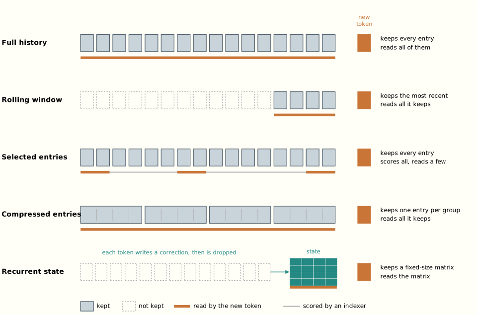
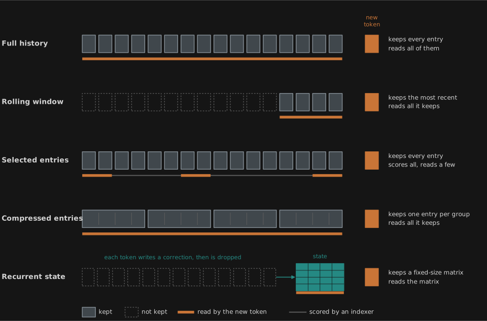
Worked example 2: a million tokens, five ways. Count what one layer keeps for a 1,000,000-token prompt, and what the next token reads. A full-attention layer keeps 1,000,000 entries and reads all of them. One of MiMo’s window layers keeps 128 and reads 128. A layer of MiniMax-M3 keeps all 1,000,000 but reads 16 blocks of 128 tokens, 2,048 positions, for each of its four groups of heads. A compressed sparse layer of DeepSeek-V4-Pro keeps about 250,000 entries, each pooled from 8 tokens at a stride of 4, and reads the 1,024 its indexer selects, plus the 128 most recent tokens uncompressed. A heavily compressed layer of the same model keeps about 7,800 entries, each pooled from 128 tokens, and reads them all. A recurrent layer of Kimi K3 keeps a matrix per head whose size does not depend on the prompt’s length, and reads that.
The example counts entries. Three qualifications apply. A sparse read does not make selection free: the indexer that chooses 1,024 entries still scores all 250,000 candidates, so its work grows with the context. A model that mixes recurrent and attention layers is not a constant-memory model: its attention layers still keep a growing cache, and with a fixed fraction of them the cost of reading a long prompt still grows quadratically, with a smaller constant. And the devices shrink different things. Grouped-query attention shares heads, MLA compresses each entry’s features, compression merges positions, and lower precision shrinks the bytes per number. DeepSeek-V4.1-Flash combines several of them and keeps 890 bytes of global cache per token.
Selection is learned retrieval
Four of the seven choose which entries to read. GLM-5.3 uses DeepSeek Sparse Attention: a small “lightning indexer” scores every earlier position for each query, and the main attention reads the 2,048 best. Its IndexShare lets one indexer serve a group of four consecutive layers. DeepSeek-V4-Pro’s compressed sparse attention applies the same kind of indexer to compressed entries, and DeepSeek-V4.1-Flash stacks two levels of it (Section 5). MiniMax-M3’s sparse attention (MSA) selects blocks of 128 positions, separately for each group of heads that share keys and values, and always includes the block that contains the query.
A selector is a second, cheaper store placed in front of the first. It scores keys, and the main attention reads only the winners. Because the choice is a hard top-k, no gradient flows through it, so the indexers learn by imitating the main attention’s distribution. The second essay describes how. What they learn can be inspected. In MiniMax’s analysis of its 109-billion-parameter research models, the indexer learns to select the first block of the sequence, which holds the “attention sink” that many heads use as a default. The new failure that selection brings is the miss: an entry the indexer did not choose cannot be read, however relevant it was.
Compression pools positions
DeepSeek-V4-Pro’s compression is learned. Each entry of its compressed sparse attention pools 8 consecutive tokens. In each of 512 channels separately, the layer computes softmax weights over the 8 tokens and takes the weighted average. Adjacent entries overlap by 4 tokens. One pooled vector serves as both key and value, shared by all 128 query heads. The heavily compressed layers pool 128 tokens per entry without overlap and attend to all of them, so they need no indexer. Each query also sees the 128 most recent tokens uncompressed, in the same softmax as the compressed entries.
In storage terms, pooling writes several positions into one entry. Within a pool the positions share a key, and attention cannot tell them apart. A fact spread across two tokens of the same pool can still be read. Two facts in one pool that a later query needs to separate cannot.
The recurrent state learns while it reads
Kimi K3 and Qwen3.8 put a recurrent layer in three of every four positions. Each keeps a matrix S per head, treated as the weights of a linear map from keys to values. For each token the layer reads the map’s current prediction for the token’s key, compares it with the token’s value, and writes the correction:
S_t=S_{t-1}+\beta_t\,(v_t-S_{t-1}k_t)\,k_t^\top .
This is one step of gradient descent on \lVert S k_t-v_t\rVert^2/2, and it is Widrow and Hoff’s rule of 1960. Schlag, Irie and Schmidhuber introduced it into linear attention so that a full memory could overwrite instead of piling up interference. The write step \beta_t, between 0 and 1, is computed from the token. Before the write, a learned decay shrinks the old state. In Qwen3.8’s Gated DeltaNet the decay is one number per head and token. In Kimi K3’s Kimi Delta Attention (KDA) it is one number per channel, so a head can keep some directions for a long time and let others fade quickly. Where Experience Goes works through an example of the rule overwriting a redefined word.
Worked example 3: per-channel forgetting. Let one row of a memory be S=(2,1), and write the value 3 under the key (1,0) with \beta=1/2. Gated DeltaNet first decays the whole row, say by 1/2, to (1,1/2). The prediction for the key is 1, the error is 2, and the write adds 1/2\times2=1 to the first coordinate: the row becomes (2,1/2). KDA can decay the two channels differently. With retention (1/2,1) the row first becomes (1,1), the write again adds 1 to the first coordinate, and the result is (2,1). The same association was corrected, and the second channel’s content survived.
What the delta rule buys over purely additive linear attention is the ability to overwrite, not capacity. Repeated writes approach the least-squares store, and Section 2 put that store’s advantage at about a factor of two. The decay sets how long contents last. In both models the gates are bounded: the write step stays between 0 and 1 and the decay between full retention and near-erasure. Section 6 returns to why those bounds matter.
What the trained hybrids do with their stores
That a model has a recurrent store does not show what it uses it for. Three recent measurements on trained models give the first answers.
Lee and colleagues placed key–value facts in a prompt to Qwen3.5-4B, a smaller relative of Qwen3.8, and asked for one of them. Then they swapped internal states between two runs that differed in the stored value. Swapping all the recurrent states moved the answer by 0.2 to 3.6 percent of the full effect. Swapping the attention caches moved it by 96 to 100 percent. Exact recall ran through the attention layers.
Afendulev and colleagues found what the recurrent states carry instead. After processing a prompt, they kept either the attention cache or the recurrent state, discarded the other, and let the model answer. With the cache alone, Qwen3.5-4B still retrieved a value from a dictionary in the prompt 89 percent of the time; with the state alone, never. Asked in the prompt to answer in another language, it complied 70 percent of the time with the state alone and 1 percent with the cache alone. A requested persona survived the same way, 49 percent against 14. Then they paired one prompt’s cache with another prompt’s state, and the answer took its content from the first and its language from the second. Kimi Linear, Moonshot’s smaller relative of K3, showed the same division. The models were far smaller than the seven, the answers short, and the results for the largest models came from a single run. Discarding one store also leaves the model in a state it never met in training, which the paired swap partly addresses.
The recurrent layers also forget quickly, by design. In Qwen3.8-27B the median recurrent head halves its contents in about 24 tokens, and the ranking of heads from fast to slow is almost the same for every document, fixed by the weights. In Kimi K3, an estimate from the weights finds that 98 percent of recurrent heads mix channels that fade to a thousandth within 64 tokens with channels that last longer.
Together these results divide the labour. The cache is the store that grows with the context, and it holds the content: values, names, the facts a later question will need. The recurrent state is the store that every token reads, and it holds a few settings that condition everything the model writes: which language, which voice. Capacity is compatible with this division but does not explain it. Afendulev and colleagues’ dictionaries held 15 to 30 entries, well within what a 128-dimensional state can hold, and they report that recall through the state fails even in minimal versions of their tasks. The division is learned.
Long context is an interference problem
As a context grows, so does the number of keys that compete with the right one. Softmax attention suppresses random competitors exponentially, but its capacity is finite at a fixed sharpness. One remedy sharpens the softmax as the context grows, multiplying \beta by a factor that grows with the logarithm of the context length. Qwen’s LogN scaling is an early instance. In Wang’s simulations with random competitors, this keeps recall nearly perfect at every length he tried, up to two million entries. Real long contexts are not random: they repeat entities, templates and phrasings, and no sharpening separates near-duplicate keys. That is one reason a model whose architecture accepts a million tokens may still fail to use them, and why the second essay treats long context as a training problem.
4. Memory along depth
The third kind of mixing runs across layers. In a standard Transformer each block reads the residual stream, computes something, and adds the result back. The residual stream is therefore a store too: within one token’s pass through the network, every block writes into it and every later block reads the sum. Two of the seven models replace this plain sum.
Several streams, mixed
DeepSeek’s Manifold-Constrained Hyper-Connections (mHC) keep four copies of the residual stream for each token, stacked as the rows of a matrix X_l. Around each block \mathcal F_l, attention or feed-forward,
X_{l+1}=B_lX_l+C_l\,\mathcal F_l(A_lX_l).
The row vector A_l mixes the four streams into the block’s input. The column vector C_l distributes the block’s output back over the streams. The matrix B_l mixes the streams among themselves. All three are computed from the current streams, so they differ from token to token. Twenty rounds of alternately normalizing its rows and columns push B_l toward a doubly stochastic matrix: one with non-negative entries whose rows and columns each sum to 1. A doubly stochastic mix conserves the total over the streams, which keeps the signal from growing or vanishing across many layers.
Worked example 4: mixing two streams. Take two scalar streams, x=(2,4), and the doubly stochastic mix with rows (3/4,1/4) and (1/4,3/4). The mixed residual is (2.5,3.5), and its total is still 6. If the block reads the average of the streams, 3, computes 6 from it, and sends half to each stream, the result is (5.5,6.5). The mixing conserved the old total; the block added new content on top. In the trained model the rows of the mixing matrix sum to 1 exactly and the columns only approximately, so the conservation is approximate.
A doubly stochastic mix has a further property. Its average channel is an ordinary residual update. The differences between the streams contract at every layer, because only a permutation preserves them all, as Li, Sha and Yang show. The extra streams are a memory that fades over depth. Zhao and colleagues measured how a trained model uses them. In DeepSeek-V4-Flash, a typical block reads about two of the four streams and writes about two. In the later half of the network the mixing is close to the identity: replacing it with the identity raised perplexity by 1.9 percent. In the earlier half the mixing matters: replacing it raised perplexity by 41.4 percent. Yet it hardly depends on the input: fixing it to its average over tokens cost 0.2 percent.
DeepSeek-V4.1-Flash changes one coefficient. Its Single-Pass mHC reads each block’s input with A_{l-1}, the mixing vector computed one step earlier, instead of A_l. With a fused kernel, the shift lets the hardware read each tile of the streams once instead of twice, and it halves the memory traffic of the original implementation. The report says the shift costs negligible quality. It was used in pretraining, so it changes the model and not only its kernel.
Attention over depth
Kimi K3’s Attention Residuals (AttnRes) replace the sum with a lookup. A layer’s input is a softmax-weighted combination of earlier representations:
h_l=\sum_i\alpha_{i\to l}\,v_i ,
where the weights come from a learned query for layer l compared with the normalized candidates. In K3 the candidates are the embedding, the completed sums of earlier groups of 12 layers, and the running sum within the current group: up to nine sources at the last layer. (The AttnRes paper calls these groups blocks.)
Worked example 5: retrieval over depth. Let two earlier representations be (1,0) and (0,2), and let the layer’s query score them at 0 and \ln 3. The softmax weights are 1/4 and 3/4, and the layer’s input is (1/4,3/2). The lookup runs over layers of the same token, not over earlier tokens.
González-Martínez and colleagues read both designs as memories over depth. AttnRes is an explicit store: a growing cache of layer outputs, read by attention. mHC is an implicit one: a fixed-size state, written by outer products. The vocabulary of Section 3 carries over unchanged, with depth in place of position. Meta’s Muse Spark Open, released in October, replaces the plain residual sum with a learned gate. The plain sum is becoming one choice among several.
Neither design feeds a later layer’s output back into an earlier layer within a pass. A store over depth lives only for the duration of one token’s computation. Whatever persists from one token to the next persists in the stores of Section 3.
5. The seven assembled
Here are the answers to Section 2’s four questions side by side, with a fifth column for how each store forgets. L is the length of the context, and d the dimension of a key.
| Store | Written by | Holds | Reading costs | Forgets |
|---|---|---|---|---|
| Feed-forward layer | training | about d clean associations with a linear readout, order d^p with a power-p nonlinearity; measured, about 2 bits per parameter | the whole layer, for every token | only when later training overwrites it |
| Experts | training | judged by total parameters, at a small penalty | a few experts, chosen by a router or, in V4-Pro’s first three layers, by a hash of the token | only when later training overwrites them |
| Engram | training, under keys fixed in advance: hashes of the last two to four tokens | a learned value per table row; tokens whose hashes collide share a row | a fixed number of lookups per token, whatever the tables’ size | only when later training overwrites it |
| Full cache | each token of the context, once | an entry per token; random keys stay separable at a fixed sharpness up to about e^{2\beta(1-\beta/d)} entries | all L entries | nothing; competitors accumulate |
| Window | each token of the context | the last 128 entries in MiMo | a fixed number of entries | everything older than the window |
| Selected entries | each token of the context | an entry per token | a scoring pass over all L, then 512 to 2,048 entries | nothing; what the indexer passes over is missed |
| Compressed entries | each group of tokens, pooled | one entry per 4 tokens (overlapping pools of 8) or per 128 in DeepSeek-V4-Pro | all entries, or a selection of them | distinctions within a pool |
| Recurrent state | each token, by a delta-rule correction | about d clean associations per head | a fixed-size matrix | by a learned decay, per head or per channel, and by overwriting |
| Residual stream | each block, within one token’s pass | one running sum | one vector | nothing is removed; later blocks add on top |
| mHC streams | each block, within one token’s pass | four running sums | a learned mix of the four | differences between the streams, which contract at every layer |
| AttnRes | each group of layers, within one token’s pass | up to nine sums in K3 | attention over the sums | distinctions between the layers of a group, which are summed |
Read down the last column. The stores written in training lose contents only when training writes over them, and that is the second essay’s subject. The stores written while reading differ in what they give up. The window gives up the old, compression gives up detail, selection gives up whatever its indexer misses, and the recurrent state gives up what decays and what is overwritten. The full cache gives up nothing, and it pays with a reading cost that grows with the context.
The seven models combine these stores as follows.
| Model | Stored / active parameters | Layers | Token mixing | Experts chosen / available |
|---|---|---|---|---|
| MiMo-V2.6-Pro | 1.02T / 42B | 70 | 60 window (128 tokens), 10 global | 8 / 384 |
| Kimi K3 | 2.8T / 104B | 93 | 69 KDA, 24 gated MLA; AttnRes over depth | 16 / 896, plus 2 shared |
| Qwen3.8 (open 2.4T checkpoint) | 2.4T / 95B | 92 | 69 Gated DeltaNet, 23 gated attention | 10 / 512, plus 1 shared |
| GLM-5.3 | not reconciled | 78 | MLA-style cache, selection of 2,048 positions | 8 / 256, plus 1 shared |
| DeepSeek-V4-Pro | 1.6T / 49B | 61 | compressed sparse and heavily compressed, with a window; mHC | 6 / 384, plus 1 shared |
| DeepSeek-V4.1-Flash | 552B, plus 196B Engram / 8B prefill, 16B decode | 20 + 20 | shared compressed sparse, hierarchical indexing; Single-Pass mHC | 6 / 384, plus 1 shared |
| MiniMax-M3 | about 428B / 23B | 60 | 3 full, 57 block-sparse | 4 / 128, plus 1 shared |
MiMo, Kimi K3, GLM-5.3, both DeepSeek models and MiniMax-M3 accept a million tokens, and Qwen3.8 extends to about the same. The parameter counts are the publishers’. GLM’s total is left open because its first-party accounting does not yet reconcile.
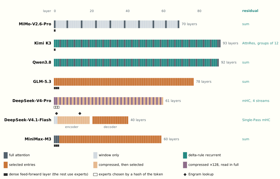
MiMo-V2.6-Pro is the most conventional of the seven. Its global layers sit at irregular positions (0, 7, 15, 23, …), and the window layers between them see 128 tokens. Locality is cheap and covers most of what a token needs; the global layers keep a path to everything else.
Kimi K3 changes all three slots at once. Its token mixer is three KDA layers for every gated MLA layer, its MLA layers use no positional encoding, and the KDA gates carry the sense of order. Its channel mixer, Stable LatentMoE, routes tokens among experts that compute in a narrower latent space. Its residual combination is AttnRes.
Qwen3.8 shares K3’s plan for the token mixer: three Gated DeltaNet layers for every attention layer. Its attention layers multiply each head’s output, channel by channel, by a sigmoid gate. The open checkpoint is the text-only counterpart of the Qwen3.8-Max service, which also reads images.
GLM-5.3 shows that a new release need not mean a new architecture. Its model card says it shares GLM-5.2’s base model and that every gain comes from post-training. The architecture it inherits pairs an MLA-style cache with DeepSeek’s sparse attention and shares each indexer across a group of four layers.
DeepSeek-V4-Pro combines two levels of compression. Its first two layers are heavily compressed, and the remaining 59 alternate between compressed sparse and heavily compressed attention. All of them add a window of recent tokens, and mHC mixes four residual streams.
DeepSeek-V4.1-Flash answers the same problem with a different design. Its causal encoder builds the decoder’s cache, so most of a prompt never passes through the decoder: that is why it uses 8 billion parameters per token while reading and 16 billion while writing. The encoder keeps three caches, at a compression of 2, each shared by six layers. The decoder keeps one uncompressed cache, computed by its first layer from the encoder’s final state and read by all twenty decoder layers. A hierarchical indexer narrows its reads: the first decoder layer chooses its own 512 positions and a pool of up to 16,384 candidates, and every fourth layer after it chooses a fresh 512 within that pool. Engram, Single-Pass mHC and 4-bit entries in the global cache complete the design.
MiniMax-M3 learns which blocks of the context to read, with three full-attention layers at the start. Its October successor, MiniMax-M3.1-Flash, has the same size and makes all 60 layers sparse.
Behind seven releases there are about five ideas: recurrent layers with a delta-rule write, mixed with attention; learned selection of what to read; learned compression of what is kept; a split between reading a prompt and writing an answer; and replacements for the plain residual sum. The October releases spread them further. Selection reached every layer of MiniMax’s model, the global layers of Step-5-Preview, StepFun’s window hybrid, and the 24 attention layers of Kimi K3.1 Pro, which keeps K3’s compressed entries and selects 2,048 of them, as GLM does. KDA-plus-MLA hybrids, which inclusionAI had adopted in August, reached 560 billion parameters in its Ling-3.1-flash. Meta replaced the residual sum. Most of these ideas are answers to one question: what a memory should be allowed to forget.
6. Depth, recurrence and what a monitor can see
Part of the case for watching a model’s reasoning rests on depth. A Transformer with a fixed number of layers can do only a bounded amount of sequential computation for each token it emits. A task that needs more has to be done in steps, and the steps appear in the text, where a monitor can read them. Recurrent layers raise the question whether that bound still holds.
“Depth” has five meanings here, and they need to be kept apart:
Architectural depth is the number of layers: 93 for Kimi K3, for every token.
The depth of an unrolled recurrence grows with the input: a recurrent layer applies one update per token, so the path from the first token to the last runs through as many updates as there are tokens.
Parallel evaluation depth can be much smaller. The recurrences in these models are affine in the state, and two consecutive updates compose into one:
(A_2,b_2)\circ(A_1,b_1)=(A_2A_1,\;A_2b_1+b_2).
Because composition is associative, L updates can be combined in a balanced tree of about \log L rounds. This is how such layers are trained in parallel.
Minimum circuit depth depends on which gates, sizes and precision one allows, and some recurrences admit much shallower circuits than their sequential form suggests.
The effective horizon, how far back the computation actually depends on its input, is a property of the trained model and the task.
The best-known constant-depth result concerns the circuit class \mathrm{TC}^0. Under its arithmetic assumptions, Merrill, Petty and Sabharwal place fixed-depth Transformers and the diagonal recurrences of Mamba-style models in it. Assuming a separation that is widely believed but unproved, the class excludes some problems of tracking a state through a sequence. Whether the delta-rule layers escape the class depends on their transition matrices. Gated DeltaNet’s update multiplies the state by \alpha_t(I-\beta_tk_tk_t^\top), which mixes coordinates and is not diagonal. Constructions that give such layers stronger state tracking, in Olmo Hybrid and in Complex KDA, widen the ranges of the gates, for instance letting the write step exceed 1 so that the factor can have a negative eigenvalue. Kimi K3’s released code, and the Transformers implementation that loads Qwen3.8, do not: the write step stays between 0 and 1. Names like “linear attention” or “delta rule” therefore do not settle where these models sit.
Hybrids have a limit of their own. Eitan, Yehudai and Maron prove that a hybrid block, whether it reads its whole cache or only the top-k entries, needs capacity of at least the square root of the domain size to compose two lookups, unless it repeats retrieval within the block. A model that retrieves once per layer may have to pay for composition in layers.
For monitoring, the important distinction is between three paths from one token to the next. The first is recurrence across positions, as in KDA and Gated DeltaNet: a numerical state carries information that the emitted text need not express. Ordinary Transformers have this path too, through their caches, so text was never the only channel between steps. The second is recurrence through depth, repeated passes through the same layers before a token is emitted. None of the seven does this. In six of eight small looped models, most answer tokens are decided at the first iteration. The third is generated text, which adds steps of computation but need not explain them faithfully.
The first measurements on these models suggest that internal and textual monitors see different things. Goodfire built simple linear probes for reward hacking from the activations of Kimi K3, GLM-5.2 and Qwen3.8, and compared them with a language model reading the whole transcript of each episode. On K3 the probes caught 33 percentage points more hacks than the transcript monitor on one benchmark and 3 more on another, and missed 7 more on a third, at the same false-positive rate. Flagging an episode when either one fired raised detection on one benchmark from 41 to 80 percent, for one percentage point more false positives. Every catch the paper shows was also visible in the text, so the probes added detection, not access to hidden reasoning. Where they fired in the middle of the reasoning, resampling from that point produced an attempted hack 29 percent of the time, against 1 percent at control points.
Monitoring is detection. Explanation is a causal account of what produced a behaviour. Depth bounds what a model can do between tokens, but it does not certify what the model did. The recurrent layers loosen that bound, in a way that depends on the algebra of their updates. The probes give monitoring a second channel.
Where the prompt went
Return to the million-token prompt. In MiMo, most of it went into the 10 global layers’ caches, where every later token can reach it, and the 60 window layers kept only the last 128 tokens. In Kimi K3, the 24 MLA layers kept a compressed entry for every token, and the 69 KDA layers folded the whole prompt into fixed-size matrices. If the trained hybrids measured so far are a guide, those matrices hold the prompt’s settings, its language and voice, while the facts stay in the cache. In DeepSeek-V4.1-Flash, the encoder read the prompt and wrote it into four caches: three compressed ones shared within the encoder, and one uncompressed one from which the decoder selects. Engram’s tables were consulted along the way. In each model the prompt was divided among stores that keep different things for different lengths of time.
These stores were not designed to hold particular contents; training filled them. The second essay takes up how: what pretraining writes and in what order, how a selector learns what to select, and what post-training changes in what was written. The stores also matter beyond engineering. Any account of a model’s states, of what persists in it and what it regulates, has to be an account of these stores, and a later essay will take that up.
Sources. The models: MiMo-V2.6-Pro (model card and technical
report, arXiv 2610.11959); Kimi K3 (model repository and technical
report, arXiv 2607.24653); Qwen3.8-2.4T-A95B (model card and
configuration); GLM-5.3 (model card) and the GLM-5 report, arXiv
2602.15763; DeepSeek-V4-Pro (model card and the V4 report, arXiv
2606.19348); DeepSeek-V4.1-Flash (model card and report, arXiv
2609.19969); MiniMax-M3 (model card) and the MSA paper, arXiv
2606.13392; MiniMax-M3.1-Flash (model card); MAI-Thinking-1 (Microsoft
AI technical report, microsoft.ai/pdf/mai-thinking-1.pdf). Components:
Vaswani et al., arXiv 1706.03762; Graves, Wayne and Danihelka,
Neural Turing Machines, arXiv 1410.5401; Zhang and Sennrich,
arXiv 1910.07467; Shazeer, arXiv 2002.05202; Su et al., arXiv
2104.09864; Ainslie et al., arXiv 2305.13245; DeepSeek-AI, arXiv
2405.04434; Shazeer et al., arXiv 1701.06538; Yang, Kautz and
Hatamizadeh, Gated Delta Networks, arXiv 2412.06464; Kimi Team,
Kimi Linear, arXiv 2510.26692; Kimi Team, Attention
Residuals, arXiv 2603.15031; Xie et al., mHC, arXiv
2512.24880; Conditional Memory via Scalable Lookup (Engram),
arXiv 2601.07372; Qwen Team, Qwen Technical Report, arXiv
2309.16609. Memory: Wang, You could have invented transformers from
memory (blog post, October 2026); Zhong et al., arXiv 2505.19488;
Kohonen, IEEE Trans. Computers C-21 (1972); Anderson, Math. Biosci. 14
(1972); Kohonen and Ruohonen, IEEE Trans. Computers C-22 (1973); Widrow
and Hoff, IRE WESCON (1960); Hopfield, PNAS 79 (1982); Amit, Gutfreund
and Sompolinsky, PRL 55 (1985); McEliece et al., IEEE Trans. IT 33
(1987); Gardner, J. Phys. A 21 (1988), via Mézard, J. Phys. A 22 (1989);
Krotov and Hopfield, arXiv 1606.01164; Demircigil et al., arXiv
1702.01929; Ramsauer et al., arXiv 2008.02217; Kanerva, Sparse
Distributed Memory (MIT Press, 1988) and Sparse Distributed
Memory and Related Models (RIACS TR 92.10, 1992); Bricken and
Pehlevan, arXiv 2111.05498; Bricken et al., arXiv 2303.11934; Sukhbaatar
et al., arXiv 1907.01470; Geva et al., arXiv 2012.14913; Schmidhuber,
Neural Computation 4 (1992); Katharopoulos et al., arXiv 2006.16236;
Schlag, Irie and Schmidhuber, arXiv 2102.11174; Nichani, Lee and Bietti,
arXiv 2412.06538; Barnfield et al., arXiv 2605.05189; Allen-Zhu and Li,
arXiv 2404.05405. Measurements on trained models: Lee et al., arXiv
2609.33093; Afendulev et al., arXiv 2609.04434; GateSight, arXiv
2610.14754; DASC, arXiv 2608.30386; Li, Sha and Yang, arXiv 2610.06653;
Zhao et al., arXiv 2609.05309; González-Martínez et al., Depth
Memory, arXiv 2610.18809. Depth and monitoring: Merrill, Petty and
Sabharwal, The Illusion of State in State-Space Models, arXiv
2404.08819; Olmo Hybrid, arXiv 2604.03444; Complex
KDA, arXiv 2609.24797; Eitan, Yehudai and Maron, arXiv 2610.25250;
Olszowiec et al., arXiv 2610.18127; Bergen et al. (Goodfire), arXiv
2609.19101. Our research notes for this essay are in the repository
under notes/research/.
This article was co-authored by Łukasz Stafiniak and Claude (Opus 5.5).